Getting started

The main functionality of h-NNE is in the HNNE class. The algorithm aims to large datasets but keep in mind that the data is loaded into memory before projection, thus you will need a server with enough RAM for your use case. Below is a simple example of projecting the CIFAR-10 dataset to two dimensions.

First let’s import the library along with torchvision which provides easy access to CIFAR-10. If you are missing some dependencies, you can install them with pip:

pip install matplotlib
pip install torchvision
pip install hnne

When all dependencies are there, you can load them:

import matplotlib.pyplot as plt
from torchvision.datasets import CIFAR10

from hnne import HNNE

Right after you can load CIFAR-10. Be aware, that the first time you load the dataset, torchvision will download it to a local datapath. This is set to ‘.’, but you can change it to point to your preferred location (e.g. /tmp).

data_path = '.'
cifar10_train = CIFAR10(root=data_path, download=True, train=True)
data = cifar10_train.data.reshape((len(cifar10_train.data), -1))
targets = cifar10_train.targets

Here comes the h-NNE part. Just load the HNNE class and call .fit_transform on the data.WARNING: malformed hyperlink target.

hnne = HNNE(verbose=True)
projection = hnne.fit_transform(data)

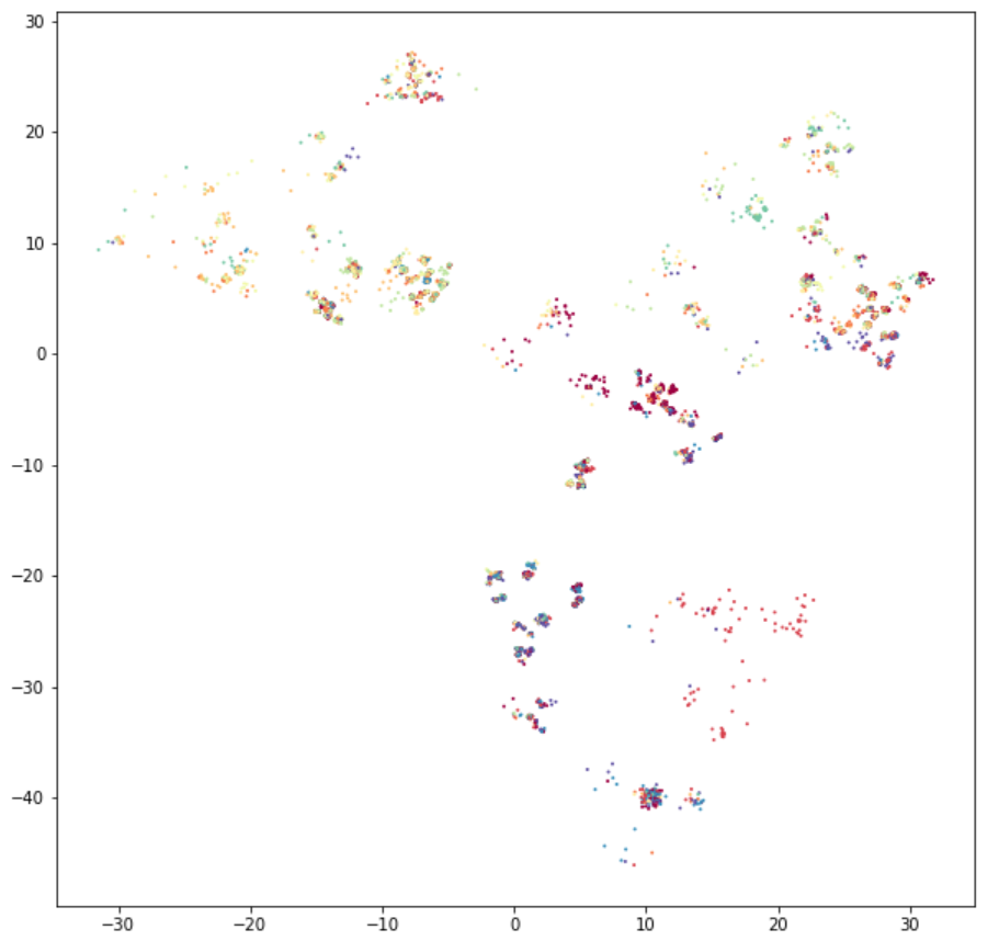
Finally, you can visualize the result with matplotlib:

plt.figure(figsize=(10, 10))
plt.scatter(*projection.T, s=1, c=targets, cmap='Spectral')
plt.show()

An extended version of this example can be found at this notebook.